Registering and aligning level 1 data

This example demonstrates how to convert AIA images to a common pointing, rescale them to a common plate scale, and remove the roll angle. This process is often referred to as “aia_prep” and the resulting data are typically referred to as level 1.5 data. In this example, we will demonstrate how to do this with aiapy. This corresponds to the aia_prep.pro procedure as described in the SDO Analysis Guide.

import matplotlib.pyplot as plt
import sunpy.map

import aiapy.data.sample as sample_data
from aiapy.calibrate import register, update_pointing

Performing multi-wavelength analysis on level 1 data can be problematic as each of the AIA channels have slightly different spatial scales and roll angles. Furthermore, the estimates of the pointing keywords (CDELT1, CDELT2, CRPIX1, CRPIX2, CROTA2) may have been improved due to limb fitting procedures after the level 1 file has been created. The Joint Science Operations Center (JSOC) stores AIA image data and metadata separately; when users download AIA data, these two data types are combined to produce a FITS file. While metadata are continuously updated at the JSOC, previously downloaded FITS files will not contain the most recent information.

Thus, before performing any multi-wavelength analyses, level 1 data should be updated to the most recent and accurate pointing and interpolated to a common grid in which the y-axis of the image is aligned with solar North.

First, let’s read a level 1 94 Å AIA image from the aiapy sample data into a Map object.

aia_map = sunpy.map.Map(sample_data.AIA_094_IMAGE)

The first step in this process is to update the metadata of the map to the most recent pointing using the aiapy.calibrate.update_pointing function. This function queries the JSOC for the most recent pointing information, updates the metadata, and returns a sunpy.map.Map with updated metadata.

aia_map_updated_pointing = update_pointing(aia_map)

If we take a look at the plate scale and rotation matrix of the map, we find that the scale is slightly off from the expected value of \(0.6''\) per pixel and that the rotation matrix has off-diagonal entries.

print(aia_map_updated_pointing.scale)
print(aia_map_updated_pointing.rotation_matrix)

SpatialPair(axis1=<Quantity 0.600109 arcsec / pix>, axis2=<Quantity 0.600109 arcsec / pix>)
[[ 0.99999712  0.0024018 ]
 [-0.0024018   0.99999712]]

We can use the aiapy.calibrate.register function to scale the image to the \(0.6''\) per pixel and derotate the image such that the y-axis is aligned with solar North.

aia_map_registered = register(aia_map_updated_pointing)

If we look again at the plate scale and rotation matrix, we should find that the plate scale in each direction is \(0.6''\) per pixel and that the rotation matrix is diagonalized. The image in aia_map_registered is now a level 1.5 data product.

print(aia_map_registered.scale)
print(aia_map_registered.rotation_matrix)

SpatialPair(axis1=<Quantity 0.6 arcsec / pix>, axis2=<Quantity 0.6 arcsec / pix>)
[[ 1.00000000e+00 -2.84766725e-20]
 [-4.62157541e-19  1.00000000e+00]]

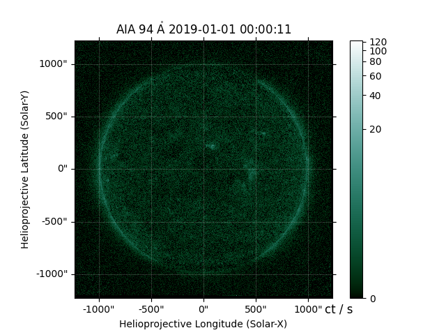
Finally, we can plot the exposure-normalized map. Note that small negative pixel values are possible because CCD images were taken with a pedestal set at ~100 DN. This pedestal is then subtracted when the JSOC pipeline performs dark (+ pedestal) subtraction and flat fielding to generate level 1 files.

fig = plt.figure()
ax = fig.add_subplot(projection=aia_map_registered)
aia_map_registered.plot(axes=ax)

plt.show()