Note
Go to the end to download the full example code
Computing wavelength response functions#
This example shows how to compute the wavelength response function of the 335 Å channel as well as explore the different properties of the telescope channels.
import astropy.time
import astropy.units as u
import matplotlib.pyplot as plt

from aiapy.response import Channel
Since AIA uses narrow-band filters, other wavelengths (outside of the nominal wavelength attributed to each filter) contribute to the image data. Computing these response functions allow us to see which other wavelengths contribute to the total intensity in each image.
First, create a aiapy.response.Channel object by specifying the
wavelength of the channel. In this case, we’ll
choose the 335 Å channel, but this same workflow
can be applied to any of the EUV or UV channels
on AIA. This may take a few seconds the first time you do
this as the most recent instrument data file will
need to be downloaded from a remote server. Subsequent
calls will know that the data has been downloaded.
c = Channel(335 * u.angstrom)
Files Downloaded:   0%|          | 0/1 [00:00<?, ?file/s]

aiapy.aia_V8_all_fullinst.genx:   0%|          | 0.00/5.43M [00:00<?, ?B/s]

aiapy.aia_V8_all_fullinst.genx:  22%|██▏       | 1.17M/5.43M [00:00<00:00, 11.6MB/s]


Files Downloaded: 100%|██████████| 1/1 [00:00<00:00,  4.92file/s]
Files Downloaded: 100%|██████████| 1/1 [00:00<00:00,  4.90file/s]
From Boerner et al. (2012), the wavelength response function is given by,
where
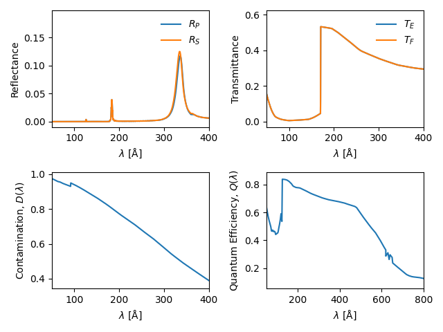
\(A_{geo}\) geometrical collecting area
\(R_P,R_S\) reflectances of primary and secondary mirrors, respectively
\(T_E, T_F\) transmission efficiency of the entrance and focal-plane filters, respectively
\(D\) contaminant transmittance of optics
\(Q\) quantum efficiency of the CCD
\(G\) gain of the CCD camera system
The aiapy.response.Channel object provides an interface to all of these
properties of the telescope. Below, we show how to plot several of these
properties as a function of wavelength.
# Reflectance
fig = plt.figure()
ax = fig.add_subplot(221)
ax.plot(c.wavelength, c.primary_reflectance, label=r"$R_P$")
ax.plot(c.wavelength, c.secondary_reflectance, label=r"$R_S$")
ax.set_ylabel(r"Reflectance")
ax.set_xlim(50, 400)
ax.set_xlabel(r"$\lambda$ [Å]")
ax.legend(frameon=False)

# Transmittance
ax = fig.add_subplot(222)
ax.plot(c.wavelength, c.entrance_filter_efficiency, label=r"$T_E$")
ax.plot(c.wavelength, c.focal_plane_filter_efficiency, label=r"$T_F$")
ax.set_ylabel(r"Transmittance")
ax.set_xlim(50, 400)
ax.set_xlabel(r"$\lambda$ [Å]")
ax.legend(frameon=False)

# Contamination
ax = fig.add_subplot(223)
ax.plot(c.wavelength, c.contamination)
ax.set_ylabel(r"Contamination, $D(\lambda)$")
ax.set_xlim(50, 400)
ax.set_xlabel(r"$\lambda$ [Å]")

# Quantumn efficiency
ax = fig.add_subplot(224)
ax.plot(c.wavelength, c.quantum_efficiency)
ax.set_ylabel(r"Quantum Efficiency, $Q(\lambda)$")
ax.set_xlim(50, 800)
ax.set_xlabel(r"$\lambda$ [Å]")
plt.tight_layout()
plt.show()

Additionally, aiapy.response.Channel provides a method for calculating
the wavelength response function using the equation above,
[1.6854788e-08 1.6595683e-08 1.6341122e-08 ... 2.5859875e-11 2.5686821e-11
 2.5515087e-11] cm2 ct / ph
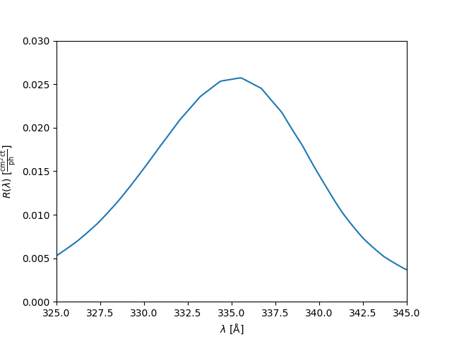
We can then plot the response as a function of wavelength.
fig = plt.figure()
ax = fig.gca()
ax.plot(c.wavelength, r)
ax.set_xlim((c.channel + [-10, 10] * u.angstrom).value)
ax.set_ylim(0, 0.03)
ax.set_xlabel(r"$\lambda$ [Å]")
ax.set_ylabel(f'$R(\\lambda)$ [{r.unit.to_string("latex")}]')
plt.show()

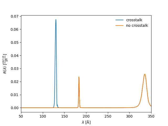
On telescopes 1, 3, and 4, both channels are always illuminated. This can lead to “crosstalk” contamination in a channel from the channel with which it shares a telescope. This impacts the 94 Å and 304 Å channels as well as the 131 Å and 335 Å channels. This effect is included by default in the wavelength response calculation. To exclude this effect,
r_no_cross = c.wavelength_response(include_crosstalk=False)
If we look at the response around 131 Å (the channel with which 335 Å shares a telescope), we can see the effect that the channel crosstalk has on the 335 Å response function.
fig = plt.figure()
ax = fig.gca()
ax.plot(c.wavelength, r, label="crosstalk")
ax.plot(c.wavelength, r_no_cross, label="no crosstalk")
ax.set_xlim(50, 350)
ax.set_xlabel(r"$\lambda$ [Å]")
ax.set_ylabel(f'$R(\\lambda)$ [{r.unit.to_string("latex")}]')
ax.legend(loc=1, frameon=False)
plt.show()

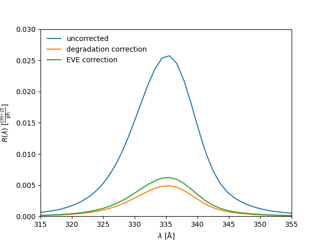
We can also incorporate various corrections to the response functions, including a time-dependent degradation correction as well as a correction based on the EVE calibration. The latter also includes the time-dependent correction. As an example, to apply the two aforementioned corrections given the degradation as of 1 January 2019,
We can then compare the two corrected response functions to the uncorrected case.
fig = plt.figure()
ax = fig.gca()
ax.plot(c.wavelength, r, label="uncorrected")
ax.plot(c.wavelength, r_time, label="degradation correction")
ax.plot(c.wavelength, r_eve, label="EVE correction")
ax.set_xlim((c.channel + [-20, 20] * u.angstrom).value)
ax.set_ylim(0, 0.03)
ax.set_xlabel(r"$\lambda$ [Å]")
ax.set_ylabel(f'$R(\\lambda)$ [{r.unit.to_string("latex")}]')
ax.legend(loc=2, frameon=False)
plt.show()

Total running time of the script: (0 minutes 7.489 seconds)