Modeling channel degradation over time

This example demonstrates how to model the degradation of the AIA channels as a function of time over the entire lifetime of the instrument.

import matplotlib.pyplot as plt
import numpy as np

import astropy.time
import astropy.units as u
from astropy.visualization import time_support

from aiapy.calibrate import degradation
from aiapy.calibrate.util import get_correction_table

# This lets you pass `astropy.time.Time` objects directly to matplotlib
time_support(format="jyear")

<astropy.visualization.time.time_support.<locals>.MplTimeConverter object at 0x795e0fc73890>

The sensitivity of the AIA channels degrade over time. Possible causes include the deposition of organic molecules from the telescope structure onto the optical elements and the decrease in detector sensitivity following (E)UV exposure. When looking at AIA images over the lifetime of the mission, it is important to understand how the degradation of the instrument impacts the measured intensity. For monitoring brightness changes over months and years, degradation correction is an important step in the data normalization process. For instance, the SDO Machine Learning Dataset (Galvez et al., 2019) includes this correction.

The AIA team models the change in transmission as a function of time (see Boerner et al., 2012) and the table of correction parameters is publicly available via the Joint Science Operations Center (JSOC).

First, fetch this correction table. We have to specify the source of the correction table. This can be either a local file or a version number of a file hosted in SSW or “jsoc” to fetch the latest version from JSOC.

correction_table = get_correction_table("JSOC")

We want to compute the degradation for each EUV channel.

aia_channels = [94, 131, 171, 193, 211, 304, 335] * u.angstrom

We can use Time to create an array of times between now and the start of the mission with a cadence of one week.

start_time = astropy.time.Time("2010-03-25T00:00:00", scale="utc")
now = astropy.time.Time.now()
time_range = start_time + np.arange(0, (now - start_time).to(u.day).value, 7) * u.day

Finally, we can use the aiapy.calibrate.degradation function to compute the degradation for a particular channel and observation time. This is modeled as the ratio of the effective area measured at a particular calibration epoch over the uncorrected effective area with a polynomial interpolation to the exact time.

degradations = {
    channel: degradation(channel, time_range, correction_table=correction_table) for channel in aia_channels
}

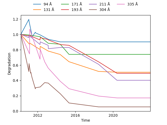
Plotting the different degradation curves as a function of time, we can easily visualize how the different channels have degraded over time.

fig = plt.figure()
ax = fig.gca()

for channel in aia_channels:
    ax.plot(time_range, degradations[channel], label=f"{channel:latex}")

ax.set_xlim(time_range[[0, -1]])
ax.legend(frameon=False, ncol=4, bbox_to_anchor=(0.5, 1), loc="lower center")
ax.set_xlabel("Time")
ax.set_ylabel("Degradation")

plt.show()